An LLM Can Infer the Rule You Forgot — in One Dimension
In this article
A few weeks ago I wrote about a world model that passes every test and still loses. The finding I was most confident about in that work was the pessimistic half: LLMs perform rule translation, not rule inference. They faithfully encode rules you tell them, and they don’t reliably infer rules you merely show them. I tried hard to repair a rule-blind model from data — proper DAgger, harvested states, two model sizes — and it stayed blind.
That conclusion was right about the setting I measured it in, and I’ve now spent a few more weeks finding out where it stops being true. The short version: move from board games to continuous control, and a current model does infer the omitted rule from a handful of examples — reliably, exactly, writing the true global rule rather than a curve fit. Then give the same rule one more dimension and the whole capability disappears, through every intervention I could design against it. The write-up is a preprint, An Omitted Mode Is a Rare Rule (arXiv:2608.17956), with the code and result artifacts open.
From board games to a cart with a wall
The reason to redo this in continuous control is that the literature there disagrees with the shape of my result. Model-based RL treats world-model error as pervasive and compounding — a bit wrong everywhere, getting worse as you roll forward. My discrete result was the opposite: error that is localized and pivotal, exactly zero almost everywhere and catastrophic on a thin set. If that geometry doesn’t survive the move to continuous state spaces, it’s a quirk of board games.
So: a cart on a track, sigmoid reward plateaus at both ends, and a wall at some position that stops the cart dead. A planner does random-shooting MPC against a synthesized Python model of the physics. The spec handed to the LLM pins the integrator exactly and simply omits the wall clause. The gate is the same idea as before — synthesize, refine against 40 sampled rollouts, accept when every transition matches to .
When the training sample happens to contain no wall contact, the result is the discrete headline reproduced in physics, end to end: the artifact passes the gate at 1.000, is exact everywhere off the wall, is fully wall-blind on probes, and the planner that trusts it drives into the phantom region, gets pinned at the wall in every episode, and replans the same doomed plan every step for the whole episode — a return of about 0.02 against the true planner’s 17.77. All 20 of those seeds, across two model sizes on disjoint sample blocks, did exactly that.
The rate that event happens at is not a mystery either. If a critical event has probability under the gate’s sampling law and the gate draws rollouts, the probability that all miss it is exactly — no asymptotics, no assumptions beyond i.i.d. rollouts. At the headline knob , so ; measured, 20 of 40 independent samples missed the wall. The interesting factor of the danger is the one you can compute in closed form.
This time, the model repairs the rule
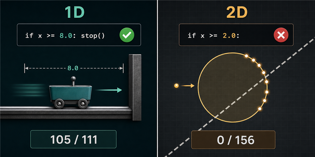
Here is where my earlier conclusion breaks. When the wall does appear in the training sample — often just a handful of contact transitions — GPT-5.x doesn’t stay blind and doesn’t fit a curve. It reads the failing transitions and writes the true global rule:
if x2 >= 8.0:
    return [8.0, 0.0]
Not a local patch around the observed contacts. The rule, with the right constant, valid everywhere.
Across the two one-dimensional instruments (the cart’s position clamp and a pendulum’s angular stop) it did this in 105 of 111 mode-containing synthesis draws. Those draws share sampled rollout blocks, so the honest unit is the block rather than the draw: every attempt was exact on 50 of 56 instrument–stream blocks, an exact 95% interval of [0.781, 0.960]. Of the six that missed, the gate caught two — superstitious local patches fitted to the observed contacts, which it refused.
That is a genuine reversal of the “translation, not inference” residual, and it’s worth saying plainly rather than burying it: a numerically manifested discontinuity is learnable from data in a way a symbolic game rule was not. A wall announces itself. Four rows out of 3,200 tilt a linear fit by twelve orders of magnitude; the LLM instead names the discontinuity and writes it down.
Then I made the rule two-dimensional
The obvious next question is whether that capability is about dimension or about discontinuity. So I built the instrument that separates them: a mover on a plane, two circular regions painted on it, and a rule that freezes the mover the moment it enters one. Same pipeline, same gate, same tolerance, same models.
What changes is the shape of the rule, not the difficulty of the physics. The wall was one number — a threshold on a single coordinate. A disc is three: two for the centre, one for the radius. (The mover’s state has four components, position and velocity on each axis, but nothing here turns on that. What matters is that the boundary is now a curve in the plane instead of a point on a line.)
Repair does not survive the move.
Zero is a number that deserves suspicion, so: those 156 draws sit over 20 distinct sampled rollout blocks, which caps the per-block repair probability at 0.168 with 95% confidence. It isn’t “never” — it’s “not once in the evidence I have, and the evidence is wide enough to make that mean something.”
What the artifacts write instead is the interesting part. The dominant failure is dimensional reduction: the disc becomes a half-plane at the right location and the wrong shape — a 1D threshold, the thing that worked on the cart, applied to a rule that isn’t one. Others fit the convex hull of the freeze positions they observed, or invent a zone around the reward landmarks. Not one of the 76 artifacts that saw a patch encoded the patch it saw.
Eight interventions, and what survives them
At this point the honest move is to attack your own explanation. If it’s curvature, flat edges should fix it. If it’s the prompt, a better prompt should fix it. So I ran eight interventions, each aimed at one candidate cause, and reported what each one changed beyond its target.
| Intervention | Repaired | What it rules out |
|---|---|---|
| Region-first prompt, 3× budget | 0/40 | the tested prompting and budget |
| Axis-aligned square, flat edges | 0/40 | boundary curvature |
| A second model family | 0/3 | one family's idiosyncrasy |
| A band in one coordinate | 0/40 | nothing — target not identifiable |
| Naming the variable the trigger reads | 0/40 | variable ambiguity |
| Mover stops inside the region | 0/40 | the interior being unobservable |
| Mover clamped to the boundary | 0/40 | the same, at matched evidence |
| Wider angular coverage of contacts | 0/40 | the evidence's coverage |
Each row is a full campaign on the same 20 sampled blocks. None of them restores repair. The fourth is recorded rather than counted: on that instrument the target is provably unidentifiable, so a zero there means nothing.
Two of those deserve a sentence. The square was the one I expected to work — if the model can write x2 >= 8.0, a box is four of those. It failed in a mirror image of the disc: artifacts wrote discs on square evidence. And the interior one was aimed at a theorem in the paper: because the patch freezes the mover at its previous position, no rollout ever occupies the region’s interior, so a sample can only ever witness entries into it. That censoring is real, and I was fairly sure it was the cause. Two campaigns lifted it — one supplying eleven times more mode evidence — and repair stayed at zero. Being wrong about your own mechanism is the part of the process that actually moves it.
What is actually missing: a located rule
The interventions are all negatives, and a negative is only worth the guarantee that its target was learnable in the first place. So, two positive controls.
From outside the pipeline: a plain algebraic least-squares circle fit — three lines of linear algebra, no prior, no language model — on exactly the evidence the synthesizer was handed. It recovers both the centre and the radius to within a tenth on 12 of 20 samples. And because the instrument lets me widen the angular spread of the contacts while holding their number fixed, I can dose the evidence until that fit succeeds on every single sample.
From inside the pipeline: replace the missing clause with a partial one that states the rule’s form and effect while withholding constants. Two levels, and they separate completely:
- Given the region’s form and its centres, with only the radius withheld — one unknown number — the synthesizer infers it exactly in 20 of 20 seeds, agreeing with the truth at IoU 1.000 on every point of the probe grid. One artifact even comments “radius inferred from the provided transitions”.
- Given the form alone, centres withheld: 0 of 20.
Put together, that places the failure precisely, and it is narrower and stranger than “2D is harder”. It is not the evidence — three lines of linear algebra recover the region from the same sample. It is not an inability to fit constants — given the location it nails the radius to float precision. It is not representational — told the rule outright, every arm writes the disc at gate 1.000 in zero refinement iterations. What the synthesizer does not do is induce a located rule: the form alone doesn’t rescue it, the form plus its location does. When the template is refused, it memorises the contacts instead of fitting them.
And this isn’t a code-versus-neural-networks story either. I ran the most favourable learned baseline I could build — the true physics pinned, with only the event function learned. On the cart it matches the code exactly: it recovers the threshold at 8.0 from four contacts, is float-exact on 3,200 held-out transitions, and passes the same gate. On the 2D instrument it recovers the near patch on 12 of 20 blocks and both patches on none. The wall is easy for everything; the circle is hard for everything that has to find it from data.
Verified, and wrong in a new way
One more result, because it’s the one that changed how I read a passing gate. Among the 1D repairs, four artifacts wrote the correct clamp and a second, invented stop on the other side — at an angle their own training rollouts never reach. Their samples cannot refute the invention, so the gate accepts them at 1.000. I re-scored all 1,034 committed artifacts against freshly drawn, disjoint acceptance samples: an independent gate caught one of those four, by the luck of its draw. What convicts the other three is a dense grid, not any rollout.
That is the whole thesis in miniature, and it has a theorem attached. Because the mode freezes the mover, there is an entire class of wrong rules that agree with the truth on every transition of every possible rollout — unfalsifiable at any sample size and any tolerance. On one instrument the larger model reliably writes exactly such a rule: nineteen of its twenty artifacts pass the gate, an independent gate, and the paper’s own probe, without encoding the region at all. The consolation is that the same argument makes them harmless: a model that is wrong only where no planner can reach costs nothing at play.
What I take from this
Sampling verification certifies your model where your samples land. That was the last paper’s point, and it survives the move to continuous control intact — including the closed-form factor for how often the sample misses what matters.
What’s new is the repair story, and it’s narrower than I’d have guessed in either direction. A capable synthesizer will recover a rule it has been shown, exactly and globally, when that rule is a threshold in one variable. It will not recover the same kind of rule when finding it means locating a region, and it doesn’t get better with a stronger prompt, more budget, flatter geometry, or more evidence — I tried all four. So the practical rule I’d give is one clause sharper than last time: coverage of the boundary is the whole game, and “the model will figure it out from the data” is a bet you can only make in one dimension. Everything with a shape, you still have to specify.
If you want the formal version — the exact gate-miss law, the volume budget that separates programs from Lipschitz models, and the unfalsifiability theorem — it’s in the preprint, and the code and every result artifact are open.
Preprint: “An Omitted Mode Is a Rare Rule” (arXiv:2608.17956) · code. Companion paper: When a Verified World Model Still Loses, and the post about it — A World Model Can Pass Every Test and Still Lose.